Step-by-Step Usage Guide
This step-by-step usage guide walks through building and running a PiperABM model. This guide is designed to help the user to understand the logic and best practices.
Step 0: Create the Model
In this first step, we import the PiperABM package and create a piperabm.Model instance and provide the parameters.
import os
import piperabm as pa

path = os.path.dirname(os.path.realpath(__file__))
model = pa.Model(
    path=path,
    seed=2,
    prices={'food': 15, 'water': 2, 'energy': 8},
    name="Example Model"
)
The model instance is now ready to be used in the subsequent steps.
Step 1: Build the Infrastructure
Now we will create the infrastructure for our model.
When you create a piperabm.Model instance, the infrastructure attribute on that instance is automatically set to a fresh piperabm.infrastructure.Infrastructure object.
Infrastructure elements include:
Market: A node where resources are bought and sold. They act as social hubs in the model. The influx of resources to the model only happens through markets. (for more info, see
add_market())Homes: Nodes where agents live and belong to. (for more info, see
add_home())Junctions: Nodes that connect edges in the network and represent a physical point in the world. (for more info, see
add_junction())Streets: Edges that are used by agents to move around the simulation world. (for more info, see
add_street())Neighborhood Access: Edges that connect homes and markets to the street network, allowing agents to access these nodes. (for more info, see
add_neighborhood_access())
The nodes are defined by their position in the world (pos), whereas edges are defined by their start and ending positions (pos_1 and pos_2). All the elements can have an optional name and are assigned a unique ID automatically, if no unique ID is given manually.
Note
ID handling policy
IDs for infrastructure elements (homes, markets, junctions, streets) are optional. If no ID is provided, PiperABM automatically assigns a unique identifier.
If a user-provided ID already exists, PiperABM will not overwrite the existing element; instead, a new unique ID is generated automatically. This behavior avoids accidental collisions during rapid prototyping, while still allowing explicit, human-readable IDs (e.g., small integers) for testing and debugging.
To build the infrastructure, we can either manually add elements:
# Option 1: Manually add all elements
# (Figure 1)
model.infrastructure.add_home(
    pos=[-60, 40],
    name='home 1',
    id=1
)
model.infrastructure.add_home(
    pos=[200, 20],
    name='home 2',
    id=2
)
model.infrastructure.add_home(
    pos=[100, -180],
    name='home 3',
    id=3
)
model.infrastructure.add_street(
    pos_1=[-60, 40],
    pos_2=[0, 0],
    name='street 1'
)
model.infrastructure.add_street(
    pos_1=[0, 0],
    pos_2=[80, 60],
    name='street 2'
)
model.infrastructure.add_street(
    pos_1=[80, 60],
    pos_2=[200, 20],
    name='street 3'
)
model.infrastructure.add_street(
    pos_1=[0, 0],
    pos_2=[100, -180],
    name='street 4'
)
model.infrastructure.add_market(
    pos=[40, -40],
    name='market',
    id=0,
    resources={'food': 150, 'water': 220, 'energy': 130}
)
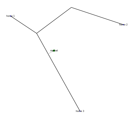
Figure 1: An example of manually defined infrastructure, after the baking process. The figure is from Manual Creation example.
… or use the methods to automatically generate the infrastructure. The generator method creates a gridworld for streets and randomlly distribute homes. It does NOT create market nodes. For more details, visit generate().
# Option 2: Automatically generate the infrastructure.
# (Figure 2)
model.infrastructure.generate(
    homes_num=20,
    grid_size=[15, 10],  # Meters
    grid_num=[6, 6],  # Meters
    imperfection_percentage=10  # Percentage of imperfection
)
model.infrastructure.add_market(
    pos=[0, 0],
    name='market',
    id=0,
    resources={'food': 150, 'water': 220, 'energy': 130}
)
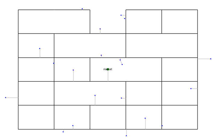
Figure 2: An example of automatically generated infrastructure, after the baking process. The grid is created with some imperfections, and a market node is added to the center of the environment and the homes are randomly placed. The figure is borrowed from Automatic Creation example.
For further details on how to load infrastructure using satellite data and maps, refer to the Working with Satellite Data.
Resources may be provided as plain dictionaries (default) or as instances of the optional Resource helper class; see the API reference for details.
Before continuing to the next step, we need to “bake” the infrastructure. The process of baking finalizes the infrastructure setup that involves applying certain graph grammars to create a physically sensinble network. For more information, please visit bake().
Note
Infrastructure lifecycle (build → bake → use)
Infrastructure construction and execution are intentionally separated in PiperABM.
Before baking, users may freely add or modify infrastructure elements.
Calling
bake()finalizes the infrastructure by applying graph-grammar and geometric rules to produce a physically consistent network.Operations that rely on a finalized network (e.g., adding agents or running the model) require the infrastructure to be baked and will raise a
ModelNotBakedErrorotherwise.Any structural change to the infrastructure after baking automatically invalidates the baked state and requires re-baking.
model.infrastructure.bake(
    proximity_radius=5,  # Meters
    search_radius=500,  # Meters
    report=True
)
When the infrastructure is baked, it is ready to be used. User can visualize the infrastructure using the show method, and by printing the infrastructure object directly, they can see a summary of the infrastructure elements.
# Print the infrastructure summary
print(model.infrastructure)

# Visualize the infrastructure
model.infrastructure.show()
The infrastructure elements are subject to degradation. There are two types of degradation:
Age: The age of the element increases over time which causes the element loose efficiency.
Usage: The more an element is used, the more it degrades.
Each degradable element has a usage_impact and age_impact attributes that are used to calculate the degradation of the element. When edges degrade, they become less efficient, therefore, it will take longer for the agents to travel through them and require more resources to do so. This is equivalent of having longer edges. This is called “adjusted length” and is calculated as follows:
The adjustement factor is calculate using the calculate_adjustment_factor method of the Degradation class. This method takes usage_impact and age_impact of the element, and by combining them with the coeff_age and coeff_usage attributes, calculates the “adjustement factor”.
By default, only the street edges are subject to degradation. However, the user can customize the degradation process by subclassing
Degradation and explicitly
injecting it into the infrastructure via set_degradation():
from piperabm.infrastructure.degradation import Degradation

class CustomDegradation(Degradation):

    def calculate_adjustment_factor(
        self, usage_impact: float, age_impact: float
    ) -> float:
        """
        Calculate adjustment factor using a custom formula.
        """
        return (
            1 + (self.infrastructure.coeff_usage * usage_impact) + (self.infrastructure.coeff_age * (age_impact ** 2))
        )

model.infrastructure.set_degradation(CustomDegradation)
For more information about custom degradation, refer to custom-degradation example.
Note
Advanced customization
Advanced users may also modify or extend the default degradation implementation
directly in the PiperABM source code (see
piperabm/infrastructure/degradation.py).
The working-directory override mechanism
provides a user-facing alternative that avoids modifying the library source code.
Step 2: Build the Society
In this step, we will create the society for our model.
Once the user create a piperabm.Model instance in Step 0, the society attribute on that instance is automatically set to a fresh piperabm.society.Society object. This instance will be used to build the society.
Society elements includes agents (as nodes) and their relationships (as edges). There are three types of relationships:
family: The agents that have same home nodes assigned are considered as a family.
neighbor: The agents that the assigned home nodes are closer than a certain distance are considered as neighbors.
friend: This type of relationship is not automatically created and can be added later by the user.
To build the society, we can either manually add agents and their relationships:
# Option 1: Manually add all elements
model.society.neighbor_radius = 500  # Meters
homes = model.infrastructure.homes  # Homes id
model.society.add_agent(
    home_id=homes[0],
    balance=1200,
    resources={'food': 15, 'water': 12, 'energy': 10},
)
model.society.add_agent(
    home_id=homes[1],
    balance=800,
    resources={'food': 15, 'water': 12, 'energy': 10},
)
model.society.add_agent(
    home_id=homes[1],
    balance=1100,
    resources={'food': 15, 'water': 12, 'energy': 10},
)
model.society.add_agent(
    home_id=homes[2],
    balance=900,
    resources={'food': 15, 'water': 12, 'energy': 10},
)
The code above is from Manual Creation example.
Note
ID handling policy
Agent IDs follow the same handling policy as infrastructure elements: IDs are optional, automatically generated if omitted, and guaranteed to be unique.
The other method is to automatically generate the society. The generator method creates a society with a given number of agents and other attributes of the society like the Gini index (a measure of inequality), average income, etc.
# Option 2: Automatically generate the society.
model.society.generate(
    num=50,
    gini_index=0.3,
    average_resources={'food': 10,'water': 10,'energy': 10},
    average_balance=1000,
)
Resources may be provided as plain dictionaries (default) or as instances of the optional Resource helper class; see the API reference for details. Agents use OODA loop, which stands for Observe, Orient, Decide, and Act as the decision-making framework. Agents observe themselves, others, and their environment, and then analyze that information using their values. The result of this decision-making a set of action, that, once executed, will impact the agents and their environment. This loop continues as long as the agetns are alive.
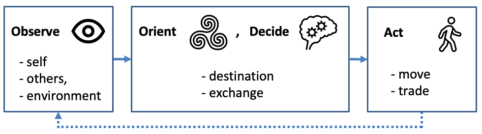
Figure 3: Agents’ satisfaction exhibits diminishing returns, plateauing once their resource inventories surpass a predefined “enough” threshold.
Agents consume resources both during travel and from their routine activities; should any of their essential resources (food, water, or energy) drop to zero, the agent is considered “dead” and is removed from the simulation, serving as a critical endpoint that reflects a failure to sustain the population under stress.
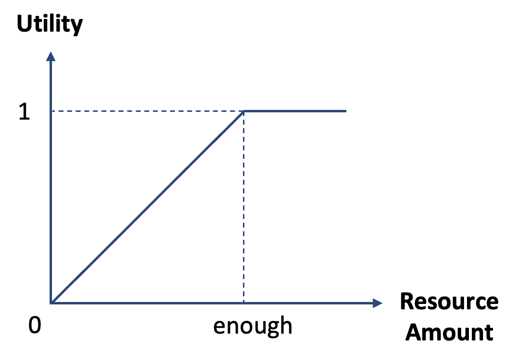
Figure 4: Agents’ satisfaction exhibits diminishing returns, plateauing once their resource inventories surpass a predefined “enough” threshold.
Agents decision-making can be customized by subclassing
DecisionMaking and explicitly injecting it
into the society via set_decision_making():
# The file name should be `decision_making.py` and it needs to be located in the wokring directory of the simulation.
from piperabm.society.decision_making import DecisionMaking

class CustomDecisionMaking(DecisionMaking):

    ...

model.society.set_decision_making(CustomDecisionMaking)
For more information about custom decision-making, refer to custom-decision-making example.
Note
Advanced customization
Advanced users may also modify or extend the default decision-making implementation
directly in the PiperABM source code (see
piperabm/society/decision_making.py).
The working-directory override mechanism
provides a user-facing alternative that avoids modifying the library source code.
Step 3: Run
When the model runs, the agents use infrastructure to interact with each other and the environment to gain access to resources. The model runs in descrete time steps, where each step represents a unit of time. During each run step, agents first perform a cost–benefit analysis to choose a destination, initially targeting the nearest market nodes to minimize travel time and resource expenditure . They then navigate through the infrastructure network using the A* algorithm, which finds the shortest path by combining actual travel costs with heuristic estimates . Upon arrival, agents may trade resources either at market nodes or with other agents present; these exchanges are resolved via the Nash Bargaining Solution, which ensures a fair division by maximizing the product of each party’s utility gain over their disagreement points. Infrastructure elements will degrade as a result of both aging usage. Agents activity will cause degradation of infrastructure elements. This feedback loop means that heavily trafficked routes become progressively slower and more costly to traverse.
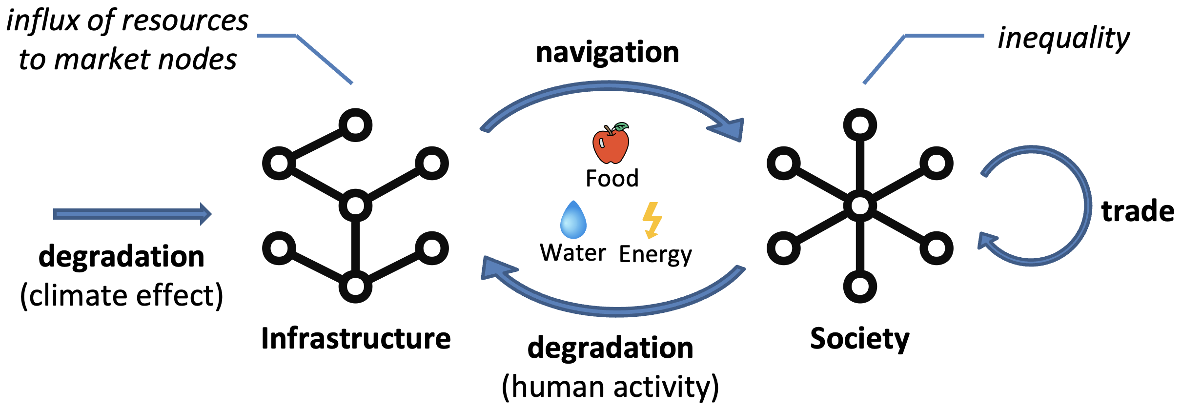
Figure 5: PiperABM models the interconnected nature of infrastructure and society networks.
The run() method of the piperabm.Model class is used for running the simulation. An example of running the model is as follows:
# Run the simulation
model.run(
    save=True,
    save_transactions=True,
    n=100,
    step_size=3600
)
Step 4: Results
When a simulation finishes, if save=True the model writes the run outputs to the
result directory in the working directory (see run()).
PiperABM saves results in a form that supports both reproducibility and fast post-hoc analysis: an initial model state (stored as NetworkX graphs) plus a sequence of per-step deltas that record how the state changes over time. These saved deltas can be replayed step-by-step without rerunning the full simulation logic, and they are also used by the measurement pipeline.
Post-hoc measurements
Measurements are intentionally decoupled from simulation execution. Using the saved deltas, the
Measurement interface can compute model-level metrics after the run completes
(e.g., accessibility and travel distance) and store them to disk for later inspection.
import os
import piperabm as pa

path = os.path.dirname(os.path.realpath(__file__))
measurement = pa.Measurement(path=path)
measurement.measure()
To load and visualize the computed measurements later:
import os
import piperabm as pa

path = os.path.dirname(os.path.realpath(__file__))
measurement = pa.Measurement(path=path)
measurement.load()
measurement.accessibility.show()
measurement.travel_distance.show()
Transactions
If enabled, transactions are recorded in a separate transactions.csv file in the result folder,
capturing exchanges between agents and/or markets.
Visualization (animation)
Animation is useful for exploratory visualization and face-validity checks. It replays the saved run data using an appropriate step-size.
import os
import piperabm as pa

path = os.path.dirname(os.path.realpath(__file__))
model = pa.Model(path=path)
model.animate()
Deterministic replay and state inspection
You can load the saved initial state and advance the model one step at a time using the saved deltas. This enables efficient inspection of internal state at arbitrary time steps without rerunning the full simulation.
import os
import piperabm as pa

path = os.path.dirname(os.path.realpath(__file__))
model = pa.Model(path=path)
model.load_initial()
for _ in range(10):
    model.push()
    print(model.society.get_balance(id=4153))
Raw graph access (NetworkX)
Both infrastructure and society are stored as NetworkX graphs and can be accessed directly for custom analysis and integration with the NetworkX ecosystem.
G_infra = model.infrastructure.G
G_soc = model.society.G
Tip
Which result workflow should I use?
Use
Measurementfor aggregate metrics across the run.Use
model.push()for step-by-step debugging and state inspection.Use
model.animate()for qualitative visualization / face-validity checks.Use
model.infrastructure.G/model.society.Gfor custom NetworkX-based analysis.